Skip to Content
CSE559AComputer Vision (Lecture 9)

CSE559A Lecture 9

Continue on ML for computer vision

Backpropagation

Computation graphs

SGD update for each parameter

wkwkηewkw_k\gets w_k-\eta\frac{\partial e}{\partial w_k}

ee is the error function.

Using the chain rule

Suppose k=1k=1, e=l(f1(x,w1),y)e=l(f_1(x,w_1),y)

Example: e=(f1(x,w1)y)2e=(f_1(x,w_1)-y)^2

So h1=f1(x,w1)=w1xh_1=f_1(x,w_1)=w^\top_1x, e=l(h1,y)=(yh1)2e=l(h_1,y)=(y-h_1)^2

ew1=eh1h1w1\frac{\partial e}{\partial w_1}=\frac{\partial e}{\partial h_1}\frac{\partial h_1}{\partial w_1} eh1=2(h1y)\frac{\partial e}{\partial h_1}=2(h_1-y) h1w1=x\frac{\partial h_1}{\partial w_1}=x ew1=2(h1y)x\frac{\partial e}{\partial w_1}=2(h_1-y)x

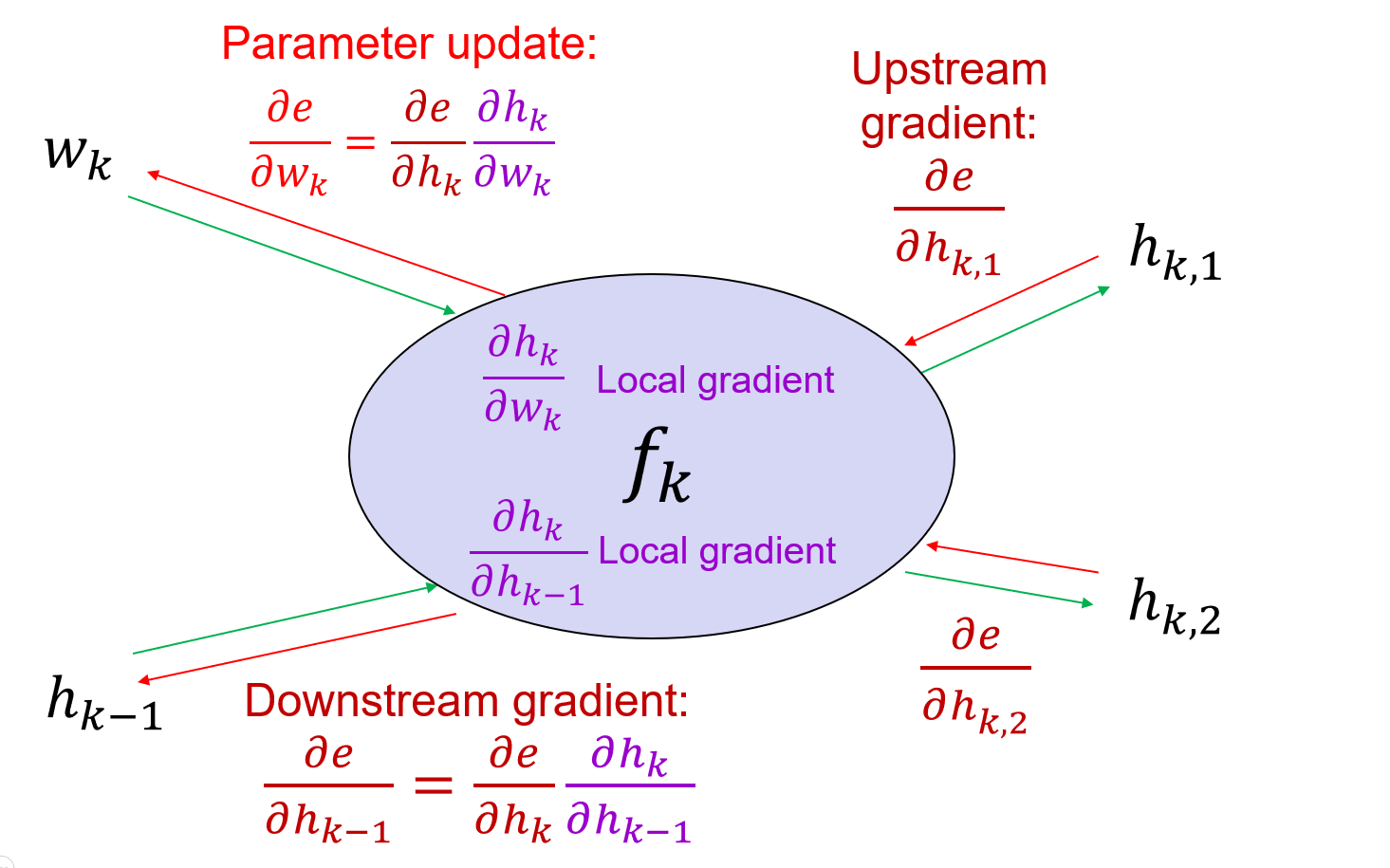
For the general cases,

ewk=ehKhKhK1hk+2hk+1hk+1hkhkwk\frac{\partial e}{\partial w_k}=\frac{\partial e}{\partial h_K}\frac{\partial h_K}{\partial h_{K-1}}\cdots\frac{\partial h_{k+2}}{\partial h_{k+1}}\frac{\partial h_{k+1}}{\partial h_k}\frac{\partial h_k}{\partial w_k}

Where the upstream gradient ehK\frac{\partial e}{\partial h_K} is known, and the local gradient hkwk\frac{\partial h_k}{\partial w_k} is known.

General backpropagation algorithm

The adding layer is the gradient distributor layer. The multiplying layer is the gradient switcher layer. The max operation is the gradient router layer.

Images of propagation

Simple example: Element-wise operation (ReLU)

f(x)=ReLU(x)=max(0,x)f(x)=ReLU(x)=max(0,x)

zx=(z1x1000z2x2000znxn)\frac{\partial z}{\partial x}=\begin{pmatrix} \frac{\partial z_1}{\partial x_1} & 0 & \cdots & 0 \\ 0 & \frac{\partial z_2}{\partial x_2} & \cdots & 0 \\ \vdots & \vdots & \ddots & \vdots \\ 0 & 0 & \cdots & \frac{\partial z_n}{\partial x_n} \end{pmatrix}

Where zixj=1\frac{\partial z_i}{\partial x_j}=1 if i=ji=j and zi>0z_i>0, otherwise zixj=0\frac{\partial z_i}{\partial x_j}=0.

When xi<0\forall x_i<0 then zx=0\frac{\partial z}{\partial x}=0 (dead ReLU)

Other examples on ppt.

Convolutional Neural Networks

Basic Convolutional layer

Flatten layer

Fully connected layer, operate on vectorized image.

With the multi-layer perceptron, the neural network trying to fit the templates.
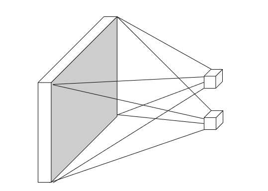
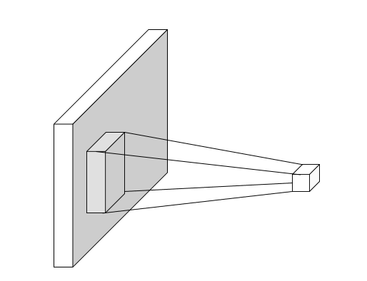
Flatten layer

Convolutional layer

Limit the receptive fields of units, tiles them over the input image, and share the weights.

Equivalent to sliding the learned filter over the image , computing dot products at each location.

Convolutional layer

Padding: Add a border of zeros around the image. (higher padding, larger output size)

Stride: The step size of the filter. (higher stride, smaller output size)

Variants 1x1 convolutions, depthwise convolutions

Backward pass

Last updated on