CSE559A Lecture 4

Practical issues with filtering

Loss of information on edges of image

• The filter window falls off the edge of the image
• Need to extrapolate
• Methods:
  • clip filter
  • wrap around (extend the image periodically)
  • copy edge (extend the image by copying the edge pixels)
  • reflect across edge (extend the image by reflecting the edge pixels)

Convolution vs Correlation

• Convolution:
  • The filter is flipped and convolved with the image

• Correlation:
  • The filter is not flipped and convolved with the image

does not matter for deep learning

scipy.signal.convolve2d(image, kernel, mode='same')
scipy.signal.correlate2d(image, kernel, mode='same')

but pytorch uses correlation for convolution, the convolution in pytorch is actually a correlation in scipy.

Frequency domain representation of linear image filters

TL;DR: It can be helpful to think about linear spatial filters in terms fro their frequency domain representation

• Fourier transform and frequency domain
• The convolution theorem

Hybrid image: More in homework 2

Human eye is sensitive to low frequencies in far field, high frequencies in near field

Change of basis from an image perspective

For vectors:

• Vector -> Invertible matrix multiplication -> New vector
• Normally we think of the standard/natural basis, with unit vectors in the direction of the axes

For images:

• Image -> Vector -> Invertible matrix multiplication -> New vector -> New image
• Standard basis is just a collection of one-hot images

Use im.flatten() to convert an image to a vector

• M is the change of basis matrix, $M^{-1}M=I$
• G is the operation we want to perform
• Vec(I) is the vectorized image

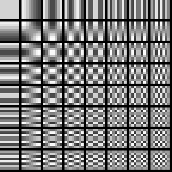
Lossy image compression (JPEG)

• JPEG is a lossy compression algorithm
• It uses the DCT (Discrete Cosine Transform) to transform the image to the frequency domain
• The DCT is a linear operation, so it can be represented as a matrix multiplication
• The JPEG algorithm then quantizes the coefficients and entropy codes them (use Huffman coding)

Thinking in frequency domain

Fourier transform

Any univariate function can be represented as a weighted sum of sine and cosine functions

• $X[k]$ is the Fourier transform of $x[n]$
• $e^{-2\pi ikn/N}$ is the basis function
• $x[n]$ is the original function

Real part:

Imaginary part:

Fourier transform stores the magnitude and phase of the sine and cosine function at each frequency

• Amplitude: encodes how much signal there is at a particular frequency
• Phase: encodes the spacial information (indirectly)
• For mathematical convenience, this is often written as a complex number

Amplitude: $A=\pm\sqrt{\text{Re}(\omega)^2+\text{Im}(\omega)^2}$

Phase: $\phi=\tan^{-1}\left(\frac{\text{Im}(\omega)}{\text{Re}(\omega)}\right)$

So use $A\sin(\omega+\phi)$ to represent the signal

Example:

$g(t)=\sin(2\pi ft)+\frac{1}{3}\sin(2\pi (3f)t)$

Fourier analysis of images

Intensity image and Fourier image

Signals can be composed.

Note: frequency domain is often visualized using a log of the absolute value of the Fourier transform

Blurring the image is to delete the high frequency components (removing the center of the frequency domain)

Convolution theorem

The Fourier transform of the convolution of two functions is the product of their Fourier transforms

• $F$ is the Fourier transform
• $*$ is the convolution

Convolution in spatial domain is equivalent to multiplication in frequency domain

• $F^{-1}$ is the inverse Fourier transform

Is convolution invertible?

• Redo the convolution in the image domain is division in the frequency domain

• This is not always possible, because $F[h]$ may be zero and we may not know the filter

Small perturbations in the frequency domain can cause large perturbations in the spatial domain and vice versa

Deconvolution is hard and a active area of research

• Even if you know the filter, it is not always possible to invert the convolution, requires strong regularization
• If you don’t know the filter, it is even harder

2D image transformations

Array slicing and image wrapping

Fast operation for extracting a subimage

• cropped image image[10:20, 10:20]
• flipped image image[::-1, ::-1]

Image wrapping allows more flexible operations

Upsampling an image

• Upsampling an image is the process of increasing the resolution of the image

Bilinear interpolation:

• Use the average of the 4 nearest pixels to determine the value of the new pixel

Other interpolation methods:

• Bicubic interpolation: Use the average of the 16 nearest pixels to determine the value of the new pixel
• Nearest neighbor interpolation: Use the value of the nearest pixel to determine the value of the new pixel