CSE559A Lecture 25

Geometry and Multiple Views

Cues for estimating Depth

Multiple Views (the strongest depth cue)

Two common settings:

Stereo vision: a pair of cameras, usually with some constraints on the relative position of the two cameras.

Structure from (camera) motion: cameras observing a scene from different viewpoints

Structure and depth are inherently ambiguous from single views.

Other hints for depth:

Occlusion
Perspective effects
Texture
Object motion
Shading
Focus/Defocus

Focus on Stereo and Multiple Views

Stereo correspondence: Given a point in one of the images, where could its corresponding points be in the other images?

Structure: Given projections of the same 3D point in two or more images, compute the 3D coordinates of that point

Motion: Given a set of corresponding points in two or more images, compute the camera parameters

A simple example of estimating depth with stereo:

Stereo: shape from “motion” between two views

We’ll need to consider:

Info on camera pose (“calibration”)
Image point correspondences

Simple stereo system

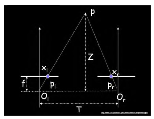
Assume parallel optical axes, known camera parameters (i.e., calibrated cameras). What is expression for Z?

Similar triangles $(p_l, P, p_r)$ and $(O_l, P, O_r)$ :

\frac{T-x_l+x_r}{Z-f}=\frac{T}{Z}

Z = \frac{f \cdot T}{x_l-x_r}

Camera Calibration

Use an scene with known geometry

Correspond image points to 3d points
Get least squares solution (or non-linear solution)

Solving unknown camera parameters:

\begin{bmatrix} su\\ sv\\ s \end{bmatrix} = \begin{bmatrix} m_{11} & m_{12} & m_{13} & m_{14}\\ m_{21} & m_{22} & m_{23} & m_{24}\\ m_{31} & m_{32} & m_{33} & m_{34} \end{bmatrix} \begin{bmatrix} X\\ Y\\ Z\\ 1 \end{bmatrix}

Method 1: Homogenous linear system. Solve for m’s entries using least squares.

\begin{bmatrix} X_1 & Y_1 & Z_1 & 1 & 0 & 0 & 0 & 0 & -u_1X_1 & -u_1Y_1 & -u_1Z_1 & -u_1 \\ 0 & 0 & 0 & 0 & X_1 & Y_1 & Z_1 & 1 & -v_1X_1 & -v_1Y_1 & -v_1Z_1 & -v_1 \\ \vdots & \vdots & \vdots & \vdots & \vdots & \vdots & \vdots & \vdots & \vdots & \vdots\\ X_n & Y_n & Z_n & 1 & 0 & 0 & 0 & 0 & -u_nX_n & -u_nY_n & -u_nZ_n & -u_n \\ 0 & 0 & 0 & 0 & X_n & Y_n & Z_n & 1 & -v_nX_n & -v_nY_n & -v_nZ_n & -v_n \end{bmatrix} \begin{bmatrix} m_{11} \\ m_{12} \\ m_{13} \\ m_{14} \\ m_{21} \\ m_{22} \\ m_{23} \\ m_{24} \\ m_{31} \\ m_{32} \\ m_{33} \\ m_{34} \end{bmatrix} = 0

Method 2: Non-homogenous linear system. Solve for m’s entries using least squares.

Advantages

Easy to formulate and solve
Provides initialization for non-linear methods

Disadvantages

Doesn’t directly give you camera parameters
Doesn’t model radial distortion
Can’t impose constraints, such as known focal length

Non-linear methods are preferred

Define error as difference between projected points and measured points
Minimize error using Newton’s method or other non-linear optimization

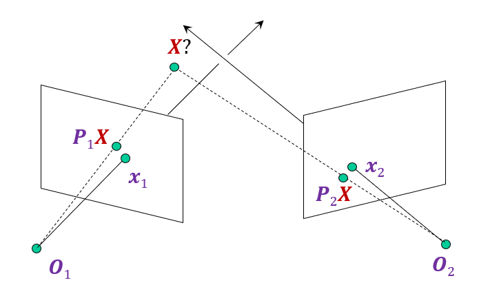
Triangulation

Given projections of a 3D point in two or more images (with known camera matrices), find the coordinates of the point

Approaches 1: Geometric approach

Find shortest segment connecting the two viewing rays and let $X$ be the midpoint of that segment

Triangulation geometric approach

Approaches 2: Non-linear optimization

Minimize error between projected point and measured point

||\operatorname{proj}(P_1 X) - x_1||_2^2 + ||\operatorname{proj}(P_2 X) - x_2||_2^2

Triangulation non-linear optimization

Approaches 3: Linear approach

$x_1\cong P_1X$ and $x_2\cong P_2X$

$x_1\times P_1X = 0$ and $x_2\times P_2X = 0$

$[x_{1_{\times}}]P_1X = 0$ and $[x_{2_{\times}}]P_2X = 0$

Rewrite as:

a\times b=\begin{bmatrix} 0 & -a_3 & a_2\\ a_3 & 0 & -a_1\\ -a_2 & a_1 & 0 \end{bmatrix} \begin{bmatrix} b_1\\ b_2\\ b_3 \end{bmatrix} =[a_{\times}]b

Using singular value decomposition, we can solve for $X$

Epipolar Geometry

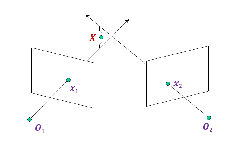
What constraints must hold between two projections of the same 3D point?

Given a 2D point in one view, where can we find the corresponding point in the other view?

Given only 2D correspondences, how can we calibrate the two cameras, i.e., estimate their relative position and orientation and the intrinsic parameters?

Key ideas:

We can answer all these questions without knowledge of the 3D scene geometry
Important to think about projections of camera centers and visual rays into the other view

Epipolar Geometry Setup

Epipolar geometry setup

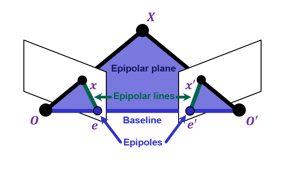
Suppose we have two cameras with centers $O,O'$

The baseline is the line connecting the origins

Epipoles $e,e'$ are where the baseline intersects the image planes, or projections of the other camera in each view

Consider a point $X$ , which projects to $x$ and $x'$

The plane formed by $X,O,O'$ is called an epipolar plane There is a family of planes passing through $O$ and $O'$

Epipolar lines are projections of the baseline into the image planes

Epipolar lines connect the epipoles to the projections of $X$ Equivalently, they are intersections of the epipolar plane with the image planes – thus, they come in matching pairs.

Application: This constraint can be used to find correspondences between points in two camera. by the epipolar line in one image, we can find the corresponding feature in the other image.

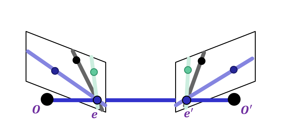
Epipolar line for converging cameras

Epipoles are finite and may be visible in the image.

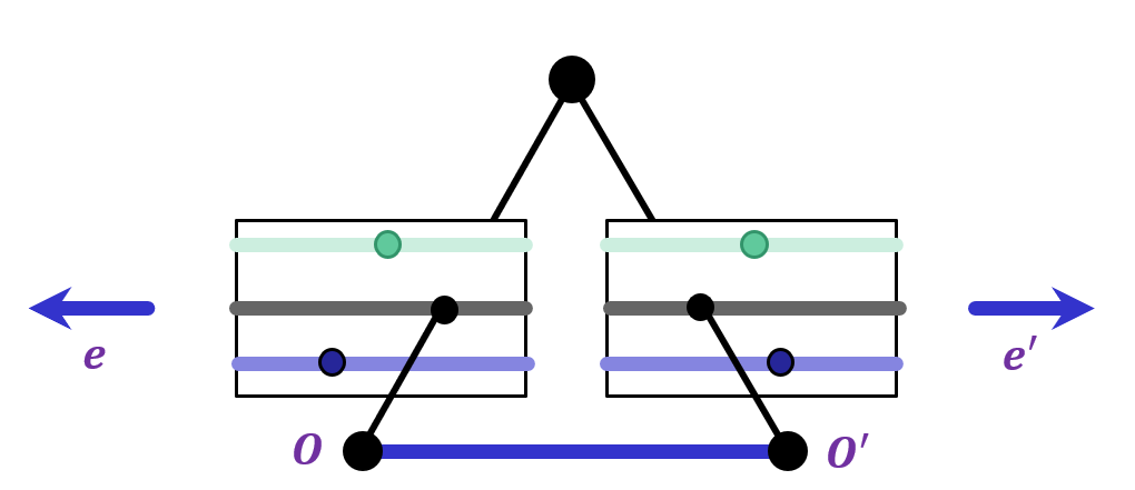
Epipolar line for parallel cameras

Epipoles are infinite, epipolar lines parallel.

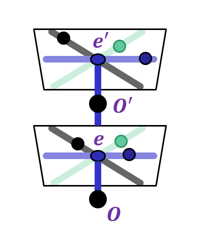
Epipolar line for perpendicular cameras

Epipole is “focus of expansion” and coincides with the principal point of the camera

Epipolar lines go out from principal point

Next class: