CSE559A Lecture 21

Continue on optical flow

The brightness constancy constraint

Given the gradients $I_x, I_y$ and $I_t$, can we uniquely recover the motion $(u,v)$?

• Suppose $(u, v)$ satisfies the constraint: $\nabla I \cdot (u,v) + I_t = 0$
• Then $\nabla I \cdot (u+u', v+v') + I_t = 0$ for any $(u', v')$ s.t. $\nabla I \cdot (u', v') = 0$
• Interpretation: the component of the flow perpendicular to the gradient (i.e., parallel to the edge) cannot be recovered!

Aperture problem

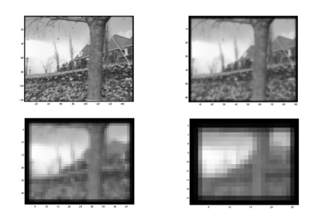
• The brightness constancy constraint is only valid for a small patch in the image
• For a large motion, the patch may look very different

Consider the barber pole illusion

Estimating optical flow (Lucas-Kanade method)

• Consider a small patch in the image
• Assume the motion is constant within the patch
• Then we can solve for the motion $(u, v)$ by minimizing the error:

How to get more equations for a pixel? Spatial coherence constraint: assume the pixel’s neighbors have the same (𝑢,𝑣) If we have 𝑛 pixels in the neighborhood, then we can set up a linear least squares system:

Lucas-Kanade flow

Let $A= \begin{bmatrix} I_x(x_1, y_1) & I_y(x_1, y_1) \\ \vdots & \vdots \\ I_x(x_n, y_n) & I_y(x_n, y_n) \end{bmatrix}$

$b = \begin{bmatrix} I_t(x_1, y_1) \\ \vdots \\ I_t(x_n, y_n) \end{bmatrix}$

$d = \begin{bmatrix} u \\ v \end{bmatrix}$

The solution is $d=(A^\top A)^{-1} A^\top b$

Lucas-Kanade flow:

• Find $(u,v)$ minimizing $\sum_{i} (I(x_i+u,y_i+v,t)-I(x_i,y_i,t-1))^2$
• use Taylor approximation of $I(x_i+u,y_i+v,t)$ for small shifts $(u,v)$ to obtain closed-form solution

Refinement for Lucas-Kanade

In some cases, the Lucas-Kanade method may not work well:

• The motion is large (larger than a pixel)
• A point does not move like its neighbors
• Brightness constancy does not hold

Iterative refinement (for large motion)

Iterative Lukas-Kanade Algorithm

1. Estimate velocity at each pixel by solving Lucas-Kanade equations
2. Warp It towards It+1 using the estimated flow field
   • use image warping techniques
3. Repeat until convergence

Iterative refinement is limited due to Aliasing

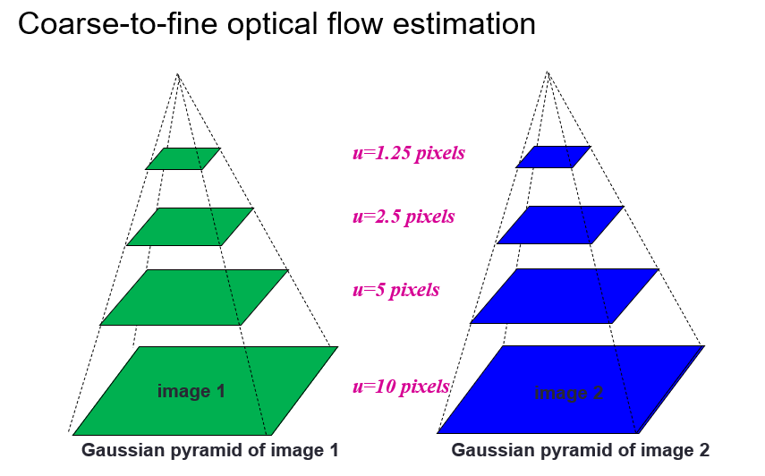
Coarse-to-fine refinement (for large motion)

• Estimate flow at a coarse level
• Refine the flow at a finer level
• Use the refined flow to warp the image
• Repeat until convergence

Representing moving images with layers (for a point may not move like its neighbors)

• The image can be decomposed into a moving layer and a stationary layer
• The moving layer is the layer that moves
• The stationary layer is the layer that does not move

SOTA models

2009

Start with something similar to Lucas-Kanade

• gradient constancy
• energy minimization with smoothing term
• region matching
• keypoint matching (long-range)

2015

Deep neural networks

• Use a deep neural network to represent the flow field
• Use synthetic data to train the network (floating chairs)

2023

GMFlow

use Transformer to model the flow field

Robust Fitting of parametric models

Challenges:

• Noise in the measured feature locations
• Extraneous data: clutter (outliers), multiple lines
• Missing data: occlusions

Least squares fitting

Normal least squares fitting

$y=mx+b$ is not a good model for the data since there might be vertical lines

Instead we use total least squares

Line parametrization: $ax+by=d$

$(a,b)$ is the unit normal to the line (i.e., $a^2+b^2=1$) $d$ is the distance between the line and the origin Perpendicular distance between point $(x_i, y_i)$ and line $ax+by=d$ (assuming $a^2+b^2=1$):

Objective function:

Solve for $d$ first: $d =a\bar{x}+b\bar{y}$ Plugging back in:

We want to find $N$ that minimizes $\|UN\|^2$ subject to $\|N\|^2= 1$ Solution is given by the eigenvector of $U^\top U$ associated with the smallest eigenvalue

Drawbacks:

• Sensitive to outliers

Robust fitting

General approach: find model parameters 𝜃 that minimize

$r(x_i;\theta)$: residual of $x_i$ w.r.t. model parameters $\theta$ $\rho_{\sigma}$: robust function with scale parameter $\sigma$, e.g., $\rho_{\sigma}(u)=\frac{u^2}{\sigma^2+u^2}$

Nonlinear optimization problem that must be solved iteratively

• Least squares solution can be used for initialization
• Scale of robust function should be chosen carefully

Drawbacks:

• Need to manually choose the robust function and scale parameter

RANSAC

Voting schemes

Random sample consensus: very general framework for model fitting in the presence of outliers

Outline:

• Randomly choose a small initial subset of points
• Fit a model to that subset
• Find all inlier points that are “close” to the model and reject the rest as outliers
• Do this many times and choose the model with the most inliers

Hough transform