CSE559A Lecture 20

Local feature descriptors

Detection: Identify the interest points

Description: Extract vector feature descriptor surrounding each interest point.

Matching: Determine correspondence between descriptors in two views

Image representation

Histogram of oriented gradients (HOG)

• Quantization
  • Grids: fast but applicable only with few dimensions
  • Clustering: slower but can quantize data in higher dimensions
• Matching
  • Histogram intersection or Euclidean may be faster
  • Chi-squared often works better
  • Earth mover’s distance is good for when nearby bins represent similar values

SIFT vector formation

Computed on rotated and scaled version of window according to computed orientation & scale

• resample the window

Based on gradients weighted by a Gaussian of variance half the window (for smooth falloff)

4x4 array of gradient orientation histogram weighted by magnitude

8 orientations x 4x4 array = 128 dimensions

Motivation: some sensitivity to spatial layout, but not too much.

For matching:

• Extraordinarily robust detection and description technique
• Can handle changes in viewpoint
  • Up to about 60 degree out-of-plane rotation
• Can handle significant changes in illumination
  • Sometimes even day vs. night
• Fast and efficient—can run in real time
• Lots of code available

SURF

• Fast approximation of SIFT idea
• Efficient computation by 2D box filters & integral images
  • 6 times faster than SIFT
• Equivalent quality for object identification

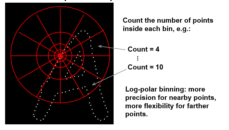
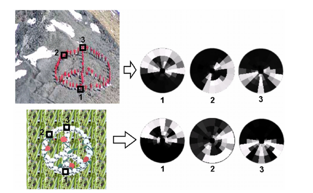
Shape context

Self-similarity Descriptor

Local feature matching

Matching

Simplest approach: Pick the nearest neighbor. Threshold on absolute distance

Problem: Lots of self similarity in many photos

Solution: Nearest neighbor with low ratio test

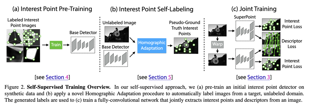
Deep Learning for Correspondence Estimation

Optical Flow

Field

Motion field: the projection of the 3D scene motion into the image Magnitude of vectors is determined by metric motion Only caused by motion

Optical flow: the apparent motion of brightness patterns in the image Magnitude of vectors is measured in pixels Can be caused by lightning

Brightness constancy constraint, aperture problem

Machine Learning Approach

• Collect examples of inputs and outputs
• Design a prediction model suitable for the task
  • Invariances, Equivariances; Complexity; Input and Output shapes and semantics
• Specify loss functions and train model
• Limitations: Requires training the model; Requires a sufficiently complete training dataset; Must re-learn known facts; Higher computational complexity

Optimization Approach

• Define properties we expect to hold for a correct solution
• Translate properties into a cost function
• Derive an algorithm to solve for the cost function
• Limitations: Often requires making overly simple assumptions on properties; Some tasks can’t be easily defined

Given frames at times $t-1$ and $t$, estimate the apparent motion field $u(x,y)$ and $v(x,y)$ between them Brightness constancy constraint: projection of the same point looks the same in every frame

Additional assumptions:

• Small motion: points do not move very far
• Spatial coherence: points move like their neighbors

Trick for solving:

Brightness constancy constraint:

Linearize the right-hand side using Taylor expansion:

Hence,