CSE559A Lecture 10

Convolutional Neural Networks

Convolutional Layer

Output feature map resolution depends on padding and stride

Padding: add zeros around the input image

Stride: the step of the convolution

Example:

1. Convolutional layer for 5x5 image with 3x3 kernel, padding 1, stride 1 (no skipping pixels)
   • Input: 5x5 image
   • Output: 3x3 feature map, (5-3+2*1)/1+1=5
2. Convolutional layer for 5x5 image with 3x3 kernel, padding 1, stride 2 (skipping pixels)
   • Input: 5x5 image
   • Output: 2x2 feature map, (5-3+2*1)/2+1=2

Learned weights can be thought of as local templates

import torch
import torch.nn as nn
 
# suppose input image is HxWx3 (assume RGB image)
 
conv_layer = nn.Conv2d(in_channels=3, # input channel, input is HxWx3
                        out_channels=64, # output channel (number of filters), output is HxWx64
                        kernel_size=3, # kernel size
                        padding=1, # padding, this ensures that the output feature map has the same resolution as the input image, H_out=H_in, W_out=W_in
                        stride=1) # stride

Usually followed by a ReLU activation function

conv_layer = nn.Conv2d(in_channels=3, out_channels=64, kernel_size=3, padding=1, stride=1)
relu = nn.ReLU()

Suppose input image is $H\times W\times K$, the output feature map is $H\times W\times L$ with kernel size $F\times F$, this takes $F^2\times K\times L\times H\times W$ parameters

Each operation $D\times (K^2C)$ matrix with $(K^2C)\times N$ matrix, assume $D$ filters and $C$ output channels.

Variants 1x1 convolutions, depthwise convolutions

1x1 convolutions

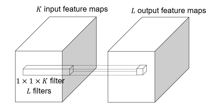
1x1 convolution: $F=1$, this layer do convolution in the pixel level, it is pixel-wise convolution for the feature.

Used to save computation, reduce the number of parameters.

Example: 3x3 conv layer with 256 channels at input and output.

Option 1: naive way:

conv_layer = nn.Conv2d(in_channels=256, out_channels=256, kernel_size=3, padding=1, stride=1)

This takes $256\times 3 \times 3\times 256=524,288$ parameters.

Option 2: 1x1 convolution:

conv_layer = nn.Conv2d(in_channels=256, out_channels=64, kernel_size=1, padding=0, stride=1)
conv_layer = nn.Conv2d(in_channels=64, out_channels=64, kernel_size=3, padding=1, stride=1)
conv_layer = nn.Conv2d(in_channels=64, out_channels=256, kernel_size=1, padding=0, stride=1)

This takes $256\times 1\times 1\times 64 + 64\times 3\times 3\times 64 + 64\times 1\times 1\times 256 = 16,384 + 36,864 + 16,384 = 69,632$ parameters.

This lose some information, but save a lot of parameters.

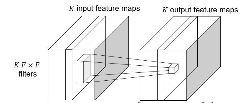
Depthwise convolutions

Depthwise convolution: $K\to K$ feature map, save computation, reduce the number of parameters.

Grouped convolutions

Self defined convolution on the feature map following the similar manner.

Backward pass

Vector-matrix form:

Suppose the kernel is 3x3, the feature map is $\ldots, x_{i-1}, x_i, x_{i+1}, \ldots$, and $\ldots, z_{i-1}, z_i, z_{i+1}, \ldots$ is the output feature map, then:

The convolution operation can be written as:

The gradient of the kernel is:

Max-pooling

Get max value in the local region.

Receptive field

The receptive field of a unit is the region of the input feature map whose values contribute to the response of that unit (either in the previous layer or in the initial image)

Architecture of CNNs

AlexNet (2012-2013)

Successor of LeNet-5, but with a few significant changes

• Max pooling, ReLU nonlinearity
• Dropout regularization
• More data and bigger model (7 hidden layers, 650K units, 60M params)
• GPU implementation (50x speedup over CPU)
  • Trained on two GPUs for a week

Key points

Most floating point operations occur in the convolutional layers.

Most of the memory usage is in the early convolutional layers.

Nearly all parameters are in the fully-connected layers.

VGGNet (2014)

GoogLeNet (2014)

ResNet (2015)

Beyond ResNet (2016 and onward): Wide ResNet, ResNeXT, DenseNet