CSE5519 Advances in Computer Vision (Topic E: 2021 and before: Deep Learning for Geometric Computer Vision)

Note

This topic is presented by Me. and will be the most detailed one for this course, perhaps.

Data set of the scene: KITTI

link to the website

PoseNet

A Convolutional Network for Real-Time 6-DOF Camera Relocalization (ICCV 2015)

Problem solving:

Camera Pose: Camera position and orientation.

link to the paper

Convolutional neural network (convnet) we train to estimate camera pose directly from a monocular image, $I$ . Our network outputs a pose vector $p$ , given by a 3D camera position $x$ and orientation represented by quaternion q:

p = [x, q]

$q$ is a quaternion, $x$ is a 3D camera position.

Arbitrary 4D values are easily mapped to legitimate rotations by normalizing them to unit length.

Regression function

Use Stochastic Gradient Descent (SGD) to optimize the network parameters.

loss(I)=\|\hat{x}-x\|_2+\beta\left\|\hat{q}-\frac{q}{\|q\|}\right\|_2

$\hat{x}$ is the estimated camera position, $x$ is the ground truth camera position, $\hat{q}$ is the estimated camera orientation, $q$ is the ground truth camera orientation.

$\beta$ is a hyperparameter that scale the loss of the camera orientation so that the network can balance on estimating the camera position and orientation approximately the same weight.

Network architecture

Based on GoogLeNet (SOTA in 2014), but with a few changes:

Replace all three softmax classifiers with affine regressors.
Insert another fully connected layer before final regressor of feature size 2048
At test time, normalize the quaternion to unit length.

Architecture


from network import Network
 
class GoogLeNet(Network):
    def setup(self):
        (self.feed('data')
             .conv(7, 7, 64, 2, 2, name='conv1')
             .max_pool(3, 3, 2, 2, name='pool1')
             .lrn(2, 2e-05, 0.75, name='norm1')
             .conv(1, 1, 64, 1, 1, name='reduction2')
             .conv(3, 3, 192, 1, 1, name='conv2')
             .lrn(2, 2e-05, 0.75, name='norm2')
             .max_pool(3, 3, 2, 2, name='pool2')
             .conv(1, 1, 96, 1, 1, name='icp1_reduction1')
             .conv(3, 3, 128, 1, 1, name='icp1_out1'))
 
        (self.feed('pool2')
             .conv(1, 1, 16, 1, 1, name='icp1_reduction2')
             .conv(5, 5, 32, 1, 1, name='icp1_out2'))
 
        (self.feed('pool2')
             .max_pool(3, 3, 1, 1, name='icp1_pool')
             .conv(1, 1, 32, 1, 1, name='icp1_out3'))
 
        (self.feed('pool2')
             .conv(1, 1, 64, 1, 1, name='icp1_out0'))
 
        (self.feed('icp1_out0', 
                   'icp1_out1', 
                   'icp1_out2', 
                   'icp1_out3')
             .concat(3, name='icp2_in')
             .conv(1, 1, 128, 1, 1, name='icp2_reduction1')
             .conv(3, 3, 192, 1, 1, name='icp2_out1'))
 
        (self.feed('icp2_in')
             .conv(1, 1, 32, 1, 1, name='icp2_reduction2')
             .conv(5, 5, 96, 1, 1, name='icp2_out2'))
 
        (self.feed('icp2_in')
             .max_pool(3, 3, 1, 1, name='icp2_pool')
             .conv(1, 1, 64, 1, 1, name='icp2_out3'))
 
        (self.feed('icp2_in')
             .conv(1, 1, 128, 1, 1, name='icp2_out0'))
 
        (self.feed('icp2_out0', 
                   'icp2_out1', 
                   'icp2_out2', 
                   'icp2_out3')
             .concat(3, name='icp2_out')
             .max_pool(3, 3, 2, 2, name='icp3_in')
             .conv(1, 1, 96, 1, 1, name='icp3_reduction1')
             .conv(3, 3, 208, 1, 1, name='icp3_out1'))
 
        (self.feed('icp3_in')
             .conv(1, 1, 16, 1, 1, name='icp3_reduction2')
             .conv(5, 5, 48, 1, 1, name='icp3_out2'))
 
        (self.feed('icp3_in')
             .max_pool(3, 3, 1, 1, name='icp3_pool')
             .conv(1, 1, 64, 1, 1, name='icp3_out3'))
 
        (self.feed('icp3_in')
             .conv(1, 1, 192, 1, 1, name='icp3_out0'))
 
        (self.feed('icp3_out0', 
                   'icp3_out1', 
                   'icp3_out2', 
                   'icp3_out3')
             .concat(3, name='icp3_out')
             .avg_pool(5, 5, 3, 3, padding='VALID', name='cls1_pool')
             .conv(1, 1, 128, 1, 1, name='cls1_reduction_pose')
             .fc(1024, name='cls1_fc1_pose')
             .fc(3, relu=False, name='cls1_fc_pose_xyz'))
 
        (self.feed('cls1_fc1_pose')
             .fc(4, relu=False, name='cls1_fc_pose_wpqr'))
 
        (self.feed('icp3_out')
             .conv(1, 1, 112, 1, 1, name='icp4_reduction1')
             .conv(3, 3, 224, 1, 1, name='icp4_out1'))
 
        (self.feed('icp3_out')
             .conv(1, 1, 24, 1, 1, name='icp4_reduction2')
             .conv(5, 5, 64, 1, 1, name='icp4_out2'))
 
        (self.feed('icp3_out')
             .max_pool(3, 3, 1, 1, name='icp4_pool')
             .conv(1, 1, 64, 1, 1, name='icp4_out3'))
 
        (self.feed('icp3_out')
             .conv(1, 1, 160, 1, 1, name='icp4_out0'))
 
        (self.feed('icp4_out0', 
                   'icp4_out1', 
                   'icp4_out2', 
                   'icp4_out3')
             .concat(3, name='icp4_out')
             .conv(1, 1, 128, 1, 1, name='icp5_reduction1')
             .conv(3, 3, 256, 1, 1, name='icp5_out1'))
 
        (self.feed('icp4_out')
             .conv(1, 1, 24, 1, 1, name='icp5_reduction2')
             .conv(5, 5, 64, 1, 1, name='icp5_out2'))
 
        (self.feed('icp4_out')
             .max_pool(3, 3, 1, 1, name='icp5_pool')
             .conv(1, 1, 64, 1, 1, name='icp5_out3'))
 
        (self.feed('icp4_out')
             .conv(1, 1, 128, 1, 1, name='icp5_out0'))
 
        (self.feed('icp5_out0', 
                   'icp5_out1', 
                   'icp5_out2', 
                   'icp5_out3')
             .concat(3, name='icp5_out')
             .conv(1, 1, 144, 1, 1, name='icp6_reduction1')
             .conv(3, 3, 288, 1, 1, name='icp6_out1'))
 
        (self.feed('icp5_out')
             .conv(1, 1, 32, 1, 1, name='icp6_reduction2')
             .conv(5, 5, 64, 1, 1, name='icp6_out2'))
 
        (self.feed('icp5_out')
             .max_pool(3, 3, 1, 1, name='icp6_pool')
             .conv(1, 1, 64, 1, 1, name='icp6_out3'))
 
        (self.feed('icp5_out')
             .conv(1, 1, 112, 1, 1, name='icp6_out0'))
 
        (self.feed('icp6_out0', 
                   'icp6_out1', 
                   'icp6_out2', 
                   'icp6_out3')
             .concat(3, name='icp6_out')
             .avg_pool(5, 5, 3, 3, padding='VALID', name='cls2_pool')
             .conv(1, 1, 128, 1, 1, name='cls2_reduction_pose')
             .fc(1024, name='cls2_fc1')
             .fc(3, relu=False, name='cls2_fc_pose_xyz'))
 
        (self.feed('cls2_fc1')
             .fc(4, relu=False, name='cls2_fc_pose_wpqr'))
 
        (self.feed('icp6_out')
             .conv(1, 1, 160, 1, 1, name='icp7_reduction1')
             .conv(3, 3, 320, 1, 1, name='icp7_out1'))
 
        (self.feed('icp6_out')
             .conv(1, 1, 32, 1, 1, name='icp7_reduction2')
             .conv(5, 5, 128, 1, 1, name='icp7_out2'))
 
        (self.feed('icp6_out')
             .max_pool(3, 3, 1, 1, name='icp7_pool')
             .conv(1, 1, 128, 1, 1, name='icp7_out3'))
 
        (self.feed('icp6_out')
             .conv(1, 1, 256, 1, 1, name='icp7_out0'))
 
        (self.feed('icp7_out0', 
                   'icp7_out1', 
                   'icp7_out2', 
                   'icp7_out3')
             .concat(3, name='icp7_out')
             .max_pool(3, 3, 2, 2, name='icp8_in')
             .conv(1, 1, 160, 1, 1, name='icp8_reduction1')
             .conv(3, 3, 320, 1, 1, name='icp8_out1'))
 
        (self.feed('icp8_in')
             .conv(1, 1, 32, 1, 1, name='icp8_reduction2')
             .conv(5, 5, 128, 1, 1, name='icp8_out2'))
 
        (self.feed('icp8_in')
             .max_pool(3, 3, 1, 1, name='icp8_pool')
             .conv(1, 1, 128, 1, 1, name='icp8_out3'))
 
        (self.feed('icp8_in')
             .conv(1, 1, 256, 1, 1, name='icp8_out0'))
 
        (self.feed('icp8_out0', 
                   'icp8_out1', 
                   'icp8_out2', 
                   'icp8_out3')
             .concat(3, name='icp8_out')
             .conv(1, 1, 192, 1, 1, name='icp9_reduction1')
             .conv(3, 3, 384, 1, 1, name='icp9_out1'))
 
        (self.feed('icp8_out')
             .conv(1, 1, 48, 1, 1, name='icp9_reduction2')
             .conv(5, 5, 128, 1, 1, name='icp9_out2'))
 
        (self.feed('icp8_out')
             .max_pool(3, 3, 1, 1, name='icp9_pool')
             .conv(1, 1, 128, 1, 1, name='icp9_out3'))
 
        (self.feed('icp8_out')
             .conv(1, 1, 384, 1, 1, name='icp9_out0'))
 
        (self.feed('icp9_out0', 
                   'icp9_out1', 
                   'icp9_out2', 
                   'icp9_out3')
             .concat(3, name='icp9_out')
             .avg_pool(7, 7, 1, 1, padding='VALID', name='cls3_pool')
             .fc(2048, name='cls3_fc1_pose')
             .fc(3, relu=False, name='cls3_fc_pose_xyz'))
 
        (self.feed('cls3_fc1_pose')
             .fc(4, relu=False, name='cls3_fc_pose_wpqr'))

Unsupervised Learning of Depth and Ego-Motion From Video

(CVPR 2017)

link to the paper

This is a method that estimates both depth and camera pose motion from a single video using CNN.

Jointly training a single-view depth CNN and a camera pose estimation CNN form unlabelled monocular video sequences.

Assumptions for PoseNet & DepthNet

The scene is static and the only motion is the camera motion.
There is no occlusion/disocclusion between the target view and the source view.
The surface is Lambertian.

View synthesis as supervision

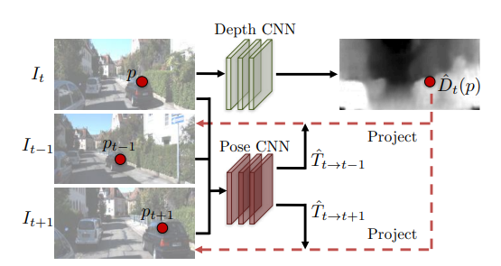
Let $I_{t-1}, I_{t}, I_{t+1}$ be three consecutive frames in the video.

First, we use the DepthNet to estimate the depth of $I_t$ to obtain $\hat{D}_t$ . We use the PoseNet to estimate the camera pose motion between $I_{t-1}$ and $I_{t+1}$ to obtain two transition vector $\hat{T}_{t\to t-1}$ and $\hat{T}_{t\to t+1}$ .

Then use the information we have from $\hat{D}_t$ and $\hat{T}_{t\to t-1}, \hat{T}_{t\to t+1}$ with frame $I_{t-1}$ and $I_{t+1}$ to synthesize the image $\hat{I}_s$ from $I_{t-1}$ and $I_{t+1}$ .

Note that $\hat{I}_s$ is the synthesized prediction for $I_t$ .

Loss function for PoseNet & DepthNet

Notice that in the training process, we can generate the supervision for PoseNet & DepthNet by using view synthesis as supervision.

View synthesis as supervision

Let $\mathcal{I}=\{I_1,I_2,I_3,\cdots,I_n\}$ be the video sequence. Note that $I_t(p)$ is the pixel value of $I_t$ at point $p$ .

The loss function generated by view synthesis is:

\mathcal{L}_{vs}=\sum_{I_s\in\mathcal{I}}\sum_{p\in I_s}\left|I_t(p)-\hat{I}_s(p)\right|

Differentiable depth image-based rendering

Assume that the transition and rotation between the frames are smooth and differentiable.

Let $p_t$ denote the pixel coordinates of $I_t$ at time $t$ . Let $K$ denote the camera intrinsic matrix. We can always obtain $p_t$ ‘s projected coordinates to our source view $p_s$ by the formula:

p_s\sim K\hat{T}_{t\to s}\hat{D}_t(p_t)K^{-1}p_t

Then we use spacial transformer network to sample continuous pixel coordinates.

Compensation for PoseNet & DepthNet

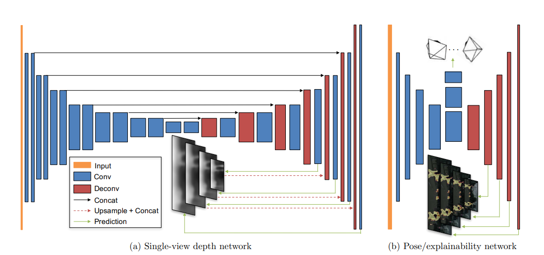
Since it’s inevitable that there are some moving objects or occlusions between the target view and the source view, in pose net we also train a few additional layers to estimate our confidence (explainability mask) of the camera motion.

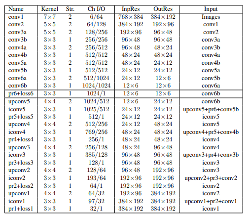
Architecture for PoseNet & DepthNet

Unsupervised Monocular Depth Estimation with Left-Right Consistency

(CVPR 2017)

link to the paper

This is a method that use pair of images as Left and Right eye to estimate depth. Increased consistency by flipping the right-left relation.

Intuition: Given a calibarated pair of binocular cameras, if we can learn a function that is able to reconstruct one image from the other, then we have learned something about the depth of the scene.

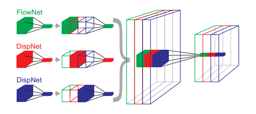
DispNet and Scene flow

link to the paper

Scene flow

Scene flow is the underlying 3D motion field that can be computed from stereo videos or RGBD videos.

Note, these 3D quantities can be computed only in the case of known camera intrinsics (i.e., $K$ matrix) and extrinsics (i.e., camera pose, translation, etc.).

Scene flow can be reconstructed only for surface points that are visible in both the left and the right frame.

Especially in the context of convolutional networks, it is particularly interesting to estimate also depth and motion in partially occluded areas

Disparity

Disparity is the difference in the x-coordinates of the same point in the left and right images.

SceneFlowNet

If there is time difference between the “left” and “right” images, by the difference between the disparity, we can estimate the scene flow, that is, non-rigid motion of the scene.

Object that have the same disparity in both images is “moving along with the camera”.

Object that is moving away, or moving toward the camera, will have higher disparity.

Assumptions for Left-right consistency Network

Lambertian surface.
No occlusion/disocclusion between the left and right image (for computing scene flow).

Loss functions for Left-right consistency Network

\mathcal{L}=\alpha_{ap}(\mathcal{L}_{ap}^l+\mathcal{L}_{ap}^r)+\alpha_{ds}(\mathcal{L}_{ds}^l+\mathcal{L}_{ds}^r)+\alpha_{lr}(\mathcal{L}_{lr}^l+\mathcal{L}_{lr}^r)

The loss function consists of three parts:

Let $N$ denote the number of pixels in the image.

Appearance matching loss

Let $I^l$ denote the left image, $I^r$ denote the right image, $\hat{L}^l$ denote the left image reconstructed from the right image.

$\hat{I}^l$ denote the left image reconstructed from the right image with the predicted disparity map $d^l$ .

The appearance matching loss for left image is:

\mathcal{L}_{ap}^l=\frac{1}{N}\sum_{p\in I^l}\alpha \frac{1-\operatorname{SSIM}(I^l(p),\hat{I}^l(p))}{2}+(1-\alpha)\left\|I^l(p)-\hat{I}^l(p)\right\|

Here $\operatorname{SSIM}$ is the structural similarity index.

link to the paper: structure similarity index

$\alpha$ is a hyperparameter that balances the importance of the structural similarity and the pixel-wise difference. In this paper, $\alpha=0.85$ .

Disparity Smoothness Loss

Let $\partial d$ denote the disparity gradient. $\partial_x d^l_p$ and $\partial_y d^l_p$ are the disparity gradient in the x and y directions respectively on the left image of pixel $p$ .

The disparity smoothness loss is:

\mathcal{L}_{ds}^l=\frac{1}{N}\sum_{p\in I^l}\left|\partial_x d^l_p\right|e^{-\left|\partial_x d^l_p\right|}+\left|\partial_y d^l_p\right|e^{-\left|\partial_y d^l_p\right|}

Left-right disparity consistency loss

Our network produces two disparity maps, $d^l$ and $d^r$ . We can use the left-right consistency loss to enforce the consistency between the two disparity maps.

\mathcal{L}_{lr}^l=\frac{1}{N}\sum_{p\in I^l}\left|d^l_p-d^r_{p+d^l_p}\right|

Architecture of Left-right consistency Network

GeoNet

Unsupervised Learning of Dense Depth, Optical Flow and Camera Pose (CVPR 2018)

Problem solving:

Depth Estimation from single monocular image.

link to the paper

link to the repository

Architecture for GeoNet

GeoNet

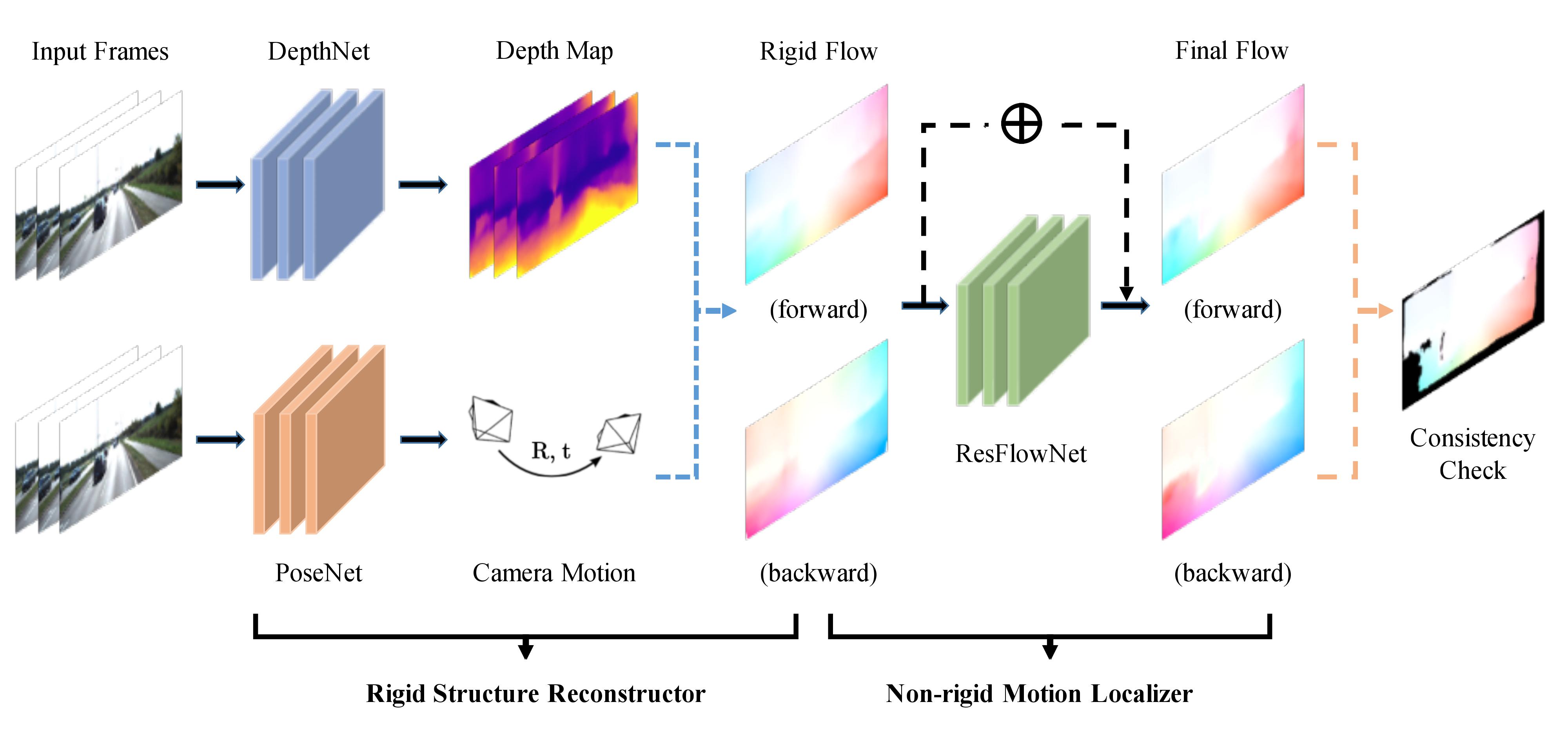
Rigid structure constructor

Combines the DepthNet and PoseNet to estimate the depth and camera pose motion from Unsupervised Learning of Depth and Ego-Motion From Video.

We denote the output of the Rigid structure constructor from frame $t$ to $s$ as $f^{rig}_{t\to s}$ . The function output is a 2D vector showing the shift of the pixel coordinates.

Recall from previous paper,

\begin{aligned} p_t+f^{rig}_{t\to s}(p_t)&=KT_{t\to s}D_t(p_t)K^{-1}p_t\\ f^{rig}_{t\to s}(p_t)&=K(T_{t\to s}D_t(p_t)+I)K^{-1}p_t-p_t \end{aligned}

Non-rigid motion localizer

Use Left-right consistency to estimate the non-rigid motion by training the ResFlowNet.

We denote the output of the Non-rigid motion localizer from frame $t$ to $s$ as $f^{res}_{t\to s}$ . SO the final full flow prediction is $f^{full}_{t\to s}=f^{res}_{t\to s}+f^{rig}_{t\to s}$ .

Let $\hat{I}^{rig}_s$ denote the inverse wrapped image from frame $s$ to $t$ . Note that $\hat{I}^{rig}_s$ is the prediction of $I_t$ from $I_s$ , using the rigid structure constructor.

Recall from previous paper, we rename the $\mathcal{L}_{ap}^l$ to $\mathcal{L}_{rw}$ .

\mathcal{L}_{rw}=\frac{1}{N}\sum_{p\in I^l}\alpha \frac{1-\operatorname{SSIM}(I^l(p),\hat{I}^{rig}_s(p))}{2}+(1-\alpha)\left\|I^l(p)-\hat{I}^{rig}_s(p)\right\|_1\tag{1}

Then we use $\mathcal{L}_{ds}$ to enforce the smoothness of the disparity map.

\mathcal{L}_{ds}=\sum_{p\in I^l}\left|\partial_x d^l_p\right|e^{-\left|\partial_x d^l_p\right|}+\left|\partial_y d^l_p\right|e^{-\left|\partial_y d^l_p\right|}=\sum_{p_t}|\nabla D(p_t)|\cdot \left(e^{-|\nabla I(p_t)|}\right)^\top\tag{2}

Replacing $\hat{I}^{rig}_s$ with $\hat{I}^{full}_s$ , in (1) and (2), we get the $\mathcal{L}_{fw}$ and $\mathcal{L}_{fs}$ for the non-rigid motion localizer.

Geometric consistency enforcement

Finally, we use an additional geometric consistency enforcement to handle non-Lambertian surfaces (e.g., metal, plastic, etc.).

This is done by additional term in the loss function.

Let $\Delta f^{full}_{t\to s}(p_t)=f^{full}_{t\to s}(p_t)-f^{full}_{s\to t}(p_t)$ .

Let $\delta(p_t)$ denote the function belows for arbitrary $\alpha,\beta>0$ :

\delta(p_t)=\begin{cases} 1 & \text{if }\|\Delta f^{full}_{t\to s}(p_t)\|_2<\max\{\alpha,\beta\|f^{full}_{t\to s}(p_t)\|_1\} \\ 0 & \text{otherwise} \end{cases}

The geometric consistency enforcement loss is:

\mathcal{L}_{gc}=\sum_{p_t}\delta(p_t)\|\Delta f^{full}_{t\to s}(p_t)\|_2

Loss function for GeoNet

Let $l$ be the set of pyramid image scales. $\langle t,s\rangle$ denote the set of all pairs of frames in the video and their inverse pairs, $t\neq s$ .

\mathcal{L}=\sum_{l}\sum_{\langle t,s\rangle}\mathcal{L}_{rw}+\lambda_{ds}\mathcal{L}_{ds}+\lambda_{fw}\mathcal{L}_{fw}+\lambda_{fs}\mathcal{L}_{fs}+\lambda_{gc}\mathcal{L}_{gc}

$\lambda_{ds},\lambda_{fw},\lambda_{fs},\lambda_{gc}$ are hyperparameters that balance the importance of the different losses.

Results for monocular depth estimation

GeoNet