CSE5313 Coding and information theory for data science (Lecture 24)

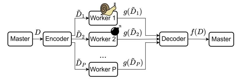
Continue on coded computing

Matrix-vector multiplication: $y=Ax$, where $A\in \mathbb{F}^{M\times N},x\in \mathbb{F}^N$

• MDS codes.
  • Recover threshold $K=M$.
• Short-dot codes.
  • Recover threshold $K\geq M$.
  • Every node receives at most $s=\frac{P-K+M}{P}$. $N$ elements of $x$.

Matrix-matrix multiplication

Problem Formulation:

• $A=[A_0 A_1\ldots A_{M-1}]\in \mathbb{F}^{L\times L}$, $B=[B_0,B_1,\ldots,B_{M-1}]\in \mathbb{F}^{L\times L}$
• $A_m,B_m$ are submatrices of $A,B$.
• We want to compute $C=A^\top B$.

Trivial solution:

• Index each worker node by $m,n\in [0,M-1]$.
• Worker node $(m,n)$ performs matrix multiplication $A_m^\top\cdot B_n$.
• Need $P=M^2$ nodes.
• No erasure tolerance.

Can we do better?

1-D MDS Method

Create $[\tilde{A}_0,\tilde{A}_1,\ldots,\tilde{A}_{S-1}]$ by encoding $[A_0,A_1,\ldots,A_{M-1}]$. with some $(S,M)$ MDS code.

Need $P=SM$ worker nodes, and index each one by $s\in [0,S-1], n\in [0,M-1]$.

Worker node $(s,n)$ performs matrix multiplication $\tilde{A}_s^\top\cdot B_n$.

Need $S-M$ responses from each column.

The recovery threshold $K=P-S+M$ nodes.

This is trivially parity check code with 1 recovery threshold.

2-D MDS Method

Encode $[A_0,A_1,\ldots,A_{M-1}]$ with some $(S,M)$ MDS code.

Encode $[B_0,B_1,\ldots,B_{M-1}]$ with some $(S,M)$ MDS code.

Need $P=S^2$ nodes.

Decodability depends on the pattern.

• Consider an $S\times S$ bipartite graph (rows on left, columns on right).
• Draw an $(i,j)$ edge if $\tilde{A}_i^\top\cdot \tilde{B}_j$ is missing
• Row $i$ is decodable if and only if the degree of $i$‘th left node $\leq S-M$.
• Column $j$ is decodable if and only if the degree of $j$‘th right node $\leq S-M$.

Peeling algorithm:

• Traverse the graph.
• If $\exists v$,$\deg v\leq S-M$, remove edges.
• Repeat.

Corollary:

• A pattern is decodable if and only if the above graph does not contain a subgraph with all degree larger than $S-M$.

Polynomial codes

Polynomial representation

Coefficient representation of a polynomial:

• $f(x)=f_dx^d+f_{d-1}x^{d-1}+\cdots+f_1x+f_0$
• Uniquely defined by coefficients $[f_d,f_{d-1},\ldots,f_0]$.

Value presentation of a polynomial:

• Theorem: A polynomial of degree $d$ is uniquely determined by $d+1$ points.
• Proof Outline: First create a polynomial of degree $d$ from the $d+1$ points using Lagrange interpolation, and show such polynomial is unique.
• Uniquely defined by evaluations $[(\alpha_1,f(\alpha_1)),\ldots,(\alpha_{d},f(\alpha_{d}))]$

Why should we want value representation?

• With coefficient representation, polynomial product takes $O(d^2)$ multiplications.
• With value representation, polynomial product takes $2d+1$ multiplications.

Definition of a polynomial code

link to paper 

Problem formulation:

We want to compute $C=A^\top B$.

Define matrix polynomials:

$p_A(x)=\sum_{i=0}^{M-1} A_i x^i$, degree $M-1$

$p_B(x)=\sum_{i=0}^{M-1} B_i x^{iM}$, degree $M(M-1)$

where each $A_i,B_i$ are matrices

We have

$\deg h(x)\leq M(M-1)+M-1=M^2-1$

Observe that

if and only if $m_1=n_1$ and $m_2=n_2$.

The coefficient of $x^{i+jM}$ is $A_i^\top B_j$.

Computing $C=A^\top B$ is equivalent to find the coefficient representation of $h(x)$.

Encoding of polynomial codes

The master choose $\omega_0,\omega_1,\ldots,\omega_{P-1}\in \mathbb{F}$.

• Note that this requires $|\mathbb{F}|\geq P$.

For every node $i\in [0,P-1]$, the master computes $\tilde{A}_i=p_A(\omega_i)$

• Equivalent to multiplying $[A_0^\top,A_1^\top,\ldots,A_{M-1}^\top]$ by Vandermonde matrix over $\omega_0,\omega_1,\ldots,\omega_{P-1}$.
• Can be speed up using FFT.

Similarly, the master computes $\tilde{B}_i=p_B(\omega_i)$ for every node $i\in [0,P-1]$.

Every node $i\in [0,P-1]$ computes and returns $c_i=p_A(\omega_i)p_B(\omega_i)$ to the master.

$c_i$ is the evaluation of polynomial $h(x)=p_A(x)p_B(x)$ at $\omega_i$.

Recall that $h(x)=\sum_{i=0}^{M-1}\sum_{j=0}^{M-1} A_i^\top B_j x^{i+jM}$.

• Computing $C=A^\top B$ is equivalent to finding the coefficient representation of $h(x)$.

Recall that a polynomial of degree $d$ can be uniquely defined by $d+1$ points.

• With $MN$ evaluations of $h(x)$, we can recover the coefficient representation for polynomial $h(x)$.

The recovery threshold $K=M^2$, independent of $P$, the number of worker nodes.

Done.

MatDot Codes

link to paper 

Problem formulation:

• We want to compute $C=A^\top B$.

• Unlike polynomial codes, we let $A=\begin{bmatrix} A_0\\ A_1\\ \vdots\\ A_{M-1} \end{bmatrix}$ and $B=\begin{bmatrix} B_0\\ B_1\\ \vdots\\ B_{M-1} \end{bmatrix}$. And $A,B\in \mathbb{F}^{L\times L}$.

• In polynomial codes, $A=\begin{bmatrix} A_0 A_1\ldots A_{M-1} \end{bmatrix}$ and $B=\begin{bmatrix} B_0 B_1\ldots B_{M-1} \end{bmatrix}$.

Key observation:

$A_m^\top$ is an $L\times \frac{L}{M}$ matrix, and $B_m$ is an $\frac{L}{M}\times L$ matrix. Hence, $A_m^\top B_m$ is an $L\times L$ matrix.

Let $C=A^\top B=\sum_{m=0}^{M-1} A_m^\top B_m$.

Let $p_A(x)=\sum_{m=0}^{M-1} A_m x^m$, degree $M-1$.

Let $p_B(x)=\sum_{m=0}^{M-1} B_m x^m$, degree $M-1$.

Both have degree $M-1$.

And $h(x)=p_A(x)p_B(x)$.

$\deg h(x)\leq M-1+M-1=2M-2$

Key observation:

• The coefficient of the term $x^{M-1}$ in $h(x)$ is $\sum_{m=0}^{M-1} A_m^\top B_m$.

Recall that $C=A^\top B=\sum_{m=0}^{M-1} A_m^\top B_m$.

Finding this coefficient is equivalent to finding the result of $A^\top B$.

Here we sacrifice the bandwidth of the network for the computational power.

General Scheme for MatDot Codes

The master choose $\omega_0,\omega_1,\ldots,\omega_{P-1}\in \mathbb{F}$.

• Note that this requires $|\mathbb{F}|\geq P$.

For every node $i\in [0,P-1]$, the master computes $\tilde{A}_i=p_A(\omega_i)$ and $\tilde{B}_i=p_B(\omega_i)$.

• $p_A(x)=\sum_{m=0}^{M-1} A_m x^m$, degree $M-1$.
• $p_B(x)=\sum_{m=0}^{M-1} B_m x^m$, degree $M-1$.

The master sends $\tilde{A}_i,\tilde{B}_i$ to node $i$.

Every node $i\in [0,P-1]$ computes and returns $c_i=p_A(\omega_i)p_B(\omega_i)$ to the master.

The master needs $\deg h(x)+1=2M-1$ evaluations to obtain $h(x)$.

• The recovery threshold is $K=2M-1$

Recap on Matrix-Matrix multiplication

$A,B\in \mathbb{F}^{L\times L}$, we want to compute $C=A^\top B$ with $P$ nodes.

Every node receives $\frac{1}{m}$ of $A$ and $\frac{1}{m}$ of $B$.

Polynomial Evaluation

Problem formulation:

• We have $K$ datasets $X_1,X_2,\ldots,X_K$.
• Want to compute some polynomial function $f$ of degree $d$ on each dataset.
  • Want $f(X_1),f(X_2),\ldots,f(X_K)$.
• Examples:
  • $X_1,X_2,\ldots,X_K$ are points in $\mathbb{F}^{M\times M}$, and $f(X)=X^8+3X^2+1$.
  • $X_k=(X_k^{(1)},X_k^{(2)})$, both in $\mathbb{F}^{M\times M}$, and $f(X)=X_k^{(1)}X_k^{(2)}$.
  • Gradient computation.

$P$ worker nodes:

• Some are stragglers, i.e., not responsive.
• Some are adversaries, i.e., return erroneous results.
• Privacy: We do not want to expose datasets to worker nodes.

Replication code

Suppose $P=(r+1)\cdot K$.

• Partition the $P$ nodes to $K$ groups of size $r+1$ each.
• Node in group $i$ computes and returns $f(X_i)$ to the master.
• Replication tolerates $r$ stragglers, or $\lfloor \frac{r}{2} \rfloor$ adversaries.

Linear codes

Recall previous linear computations (matrix-vector):

• $[\tilde{A}_1,\tilde{A}_2,\tilde{A}_3]=[A_1,A_2,A_1+A_2]$ is the corresponding codeword of $[A_1,A_2]$.
• Every worker node $i$ computes $f(\tilde{A}_i)=\tilde{A}_i x$.
• $[\tilde{A}_1x, \tilde{A}_2x, \tilde{A}_3x]=[A_1x,A_2x,A_1x+A_2x]$ is the corresponding codeword of $[A_1x,A_2x]$.
  • This enables to decode $[A_1x,A_2x]$ from $[\tilde{A}_1x,\tilde{A}_2x,\tilde{A}_3 x]$.

However, $f$ is a polynomial of degree $d$, not a linear transformation unless $d=1$.

• $f(cX)\neq cf(X)$, where $c$ is a constant.
• $f(X_1+X_2)\neq f(X_1)+f(X_2)$.

Our goal is to create an encoder/decode such that:

• Linear encoding: is the codeword of $[X_1,X_2,\ldots,X_K]$ for some linear code.
  • i.e., $[\tilde{X}_1,\tilde{X}_2,\ldots,\tilde{X}_K]=[X_1,X_2,\ldots,X_K]G$ for some generator matrix $G$.
  • Every $\tilde{X}_i$ is some linear combination of $X_1,\ldots,X_K$.
• The $f(X_i)$ are decodable from some subset of $f(\tilde{X}_i)$‘s.
  • Some of coded results are missing, erroneous.
• $X_i$’s are kept private.

Lagrange Coded Computing

Let $\ell(z)$ be a polynomial whose evaluations at $\omega_1,\ldots,\omega_{K}$ are $X_1,\ldots,X_K$.

• That is, $\ell(\omega_i)=X_i$ for every $\omega_i\in \mathbb{F}, i\in [K]$.

Some example constructions:

Given $X_1,\ldots,X_K$ with corresponding $\omega_1,\ldots,\omega_K$

• $\ell(z)=\sum_{i=1}^K X_iL_i(z)$, where $L_i(z)=\prod_{j\in[K],j\neq i} \frac{z-\omega_j}{\omega_i-\omega_j}=\begin{cases} 0 & \text{if } j\neq i \\ 1 & \text{if } j=i \end{cases}$.

Then every $f(X_i)=f(\ell(\omega_i))$ is an evaluation of polynomial $f\circ \ell(z)$ at $\omega_i$.

If the master obtains the composition $h=f\circ \ell$, it can obtain every $f(X_i)=h(\omega_i)$.

Goal: The master wished to obtain the polynomial $h(z)=f(\ell(z))$.

Intuition:

• Encoding is performed by evaluating $\ell(z)$ at $\alpha_1,\ldots,\alpha_P\in \mathbb{F}$, and $P>K$ for redundancy.
• Nodes apply $f$ on an evaluation of $\ell$ and obtain an evaluation of $h$.
• The master receives some potentially noisy evaluations, and finds $h$.
• The master evaluates $h$ at $\omega_1,\ldots,\omega_K$ to obtain $f(X_1),\ldots,f(X_K)$.

Encoding for Lagrange coded computing

Need polynomial $\ell(z)$ such that:

• $X_k=\ell(\omega_k)$ for every $k\in [K]$.

Having obtained such $\ell$ we let $\tilde{X}_i=\ell(\alpha_i)$ for every $i\in [P]$.

$span{\tilde{X}_1,\tilde{X}_2,\ldots,\tilde{X}_P}=span{\ell_1(x),\ell_2(x),\ldots,\ell_P(x)}$.

Want $X_k=\ell(\omega_k)$ for every $k\in [K]$.

Tool: Lagrange interpolation.

• $\ell_k(z)=\prod_{i\neq k} \frac{z-\omega_j}{\omega_k-\omega_j}$.
• $\ell_k(\omega_k)=1$ and $\ell_k(\omega_k)=0$ for every $j\neq k$.
• $\deg \ell_k(z)=K-1$.

Let $\ell(z)=\sum_{k=1}^K X_k\ell_k(z)$.

• $\deg \ell\leq K-1$.
• $\ell(\omega_k)=X_k$ for every $k\in [K]$.

Let $\tilde{X}_i=\ell(\alpha_i)=\sum_{k=1}^K X_k\ell_k(\alpha_i)$.

Every $\tilde{X}_i$ is a linear combination of $X_1,\ldots,X_K$.

This $G$ is called a Lagrange matrix with respect to

• $\omega_1,\ldots,\omega_K$. (interpolation points)
• $\alpha_1,\ldots,\alpha_P$. (evaluation points)

Continue next lecture